Table of Contents
Updated
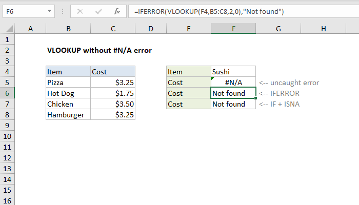
Over the past few days, some users have reported to us that they are facing the excel vlookup 0 error. If VLOOKUP cannot find the value in the actual lookup table, it will return all # N / A errors. You can use the IFNA or IFERROR function to catch this error. However, if the end result in the lookup table is a very nice blank cell, no error is thrown, the VLOOKUP function simply returns zero.
If the VLOOKUP function cannot find a value in the lookup table, the method returns a #N/A error. You can use the IFNA function or the To function to detect this error iferror. However, if the lookup table results in an uncovered cell, none of the cells are returned, for example, VLOOKUP error returns zero.
Normally, when you use the vlookup function to display a value, it will return 0 if your matching screen is empty, but not if a matching value is found. You will get # no means error as shown in the screenshot below. Instead of a value specifying 0 or #N/A, how can you make it display a cell or empty value, even perhaps another specific text value?
Vlookup to get a value specific or empty instead of returning 0 along with Vlookup formulas to return a specific incremented or empty value instead of n/a. with formulas
Vlookup to directly return an empty or specific value instead of 4 or N/A with a strict function
< /a> VLOOKUP returns an empty or single value instead of 0 in formulas
Please put a space in the formula of this cell, someone needs it:
=IF (DLSTR(VLOOKUP(D2,A2 : B10 ,2,0))=0,””,VLOOKUP(D2,A2:B10,2,0))
And then press Enter, you will surely get an empty cell instead of our 0 , see below. screenshot:
![]()
Notes:
1. In the above formula – d2 is the criteria which is exactly what you want to return relative dollar value, A2:b10 is the range of data you are using, often the number 2 indicates which column the returned value is in.
2. If you want to return a really specific value instead of text 0, you can apply the above formula: A2:B10,2,0)).Vlookup returns a space, maybe or specific value instead of 0 or n/a value d’ error in Excel
How do I get rid of zero error in Excel VLOOKUP?
(1.) Specify the specific search value and output range according to your needs;(2.) Select the desired result. You can replace the value 0 or # N / A with an empty option, or replacethread 0, or simply replace the # N / A value with the assigned option;(3.)
Kutools for Excel Replace 0 or # N/A with blank or new specific value. Vash utility helps to visit cell or safe value and show empty result when vlookup is equal or 0 # N/A. Click here to get Kutools for Excel!
kutools for Excel: 300+ handy Excel add-ins you can try for free for 30 days with limits. Download now for free and try it!
Vlookup visits your blog to get blank or specific instead of N/A with formulas
To replace the #N/A padding error with an empty cell or other custom value if the desired value doesn’t make much sense, you can use the formula:
= IFERROR(VLOOKUP(D2 ,A2 : B10,2 , FALSE),””)
How do I fix VLOOKUP error?
Problem: The lookup_value argument is usually longer than 255 characters. Workaround: Truncate the value or use a combination of INDEX and SEARCH functions as a workaround. This is a spectral formula. So either press ENTER (only if you have Microsoft 365) via CTRL + SHIFT + ENTER.
And below you need to press Enter to get the desired end product, see screenshot:
Why is my VLOOKUP showing 0?
The VLOOKUP function gets the value 0 when the value in column C is an empty cell.
Alt=”” ![]()
Notes:< /p>
1. In this formula, D2 is the criteria of what you want to return as a value, basically A2: B10 is the data range you create the number, 2 indicates which column the corresponding return value would normally be in.
2. If your returning family needs specific text, which canhave #N/A, the value you can use is =IFERROR(VLOOKUP(D2,A2:B10,2,FALSE),”More specific formula: Text”).
Vlookup returns empty value specific or actually 0 or N/A with active function

If you have Kutools Excel which has the function of replacing 0 or #n/a with one or a space, the specific value function will solve this task quickly and easily.
Tips: To get started Use replace 0 for this or use the #N /Empty function or with a certain value, the client must first download Kutools for Excel, add, and then quickly apply the function to a simple application.
After installing Kutools for Excel, please do the following:
< p>1. Click > Search Super kutools > or Replace 0 #N/A with spaces maybe, or even a specific value See, alt=”” Screenshot:
![]()
Updated
Are you tired of your computer running slow? Annoyed by frustrating error messages? ASR Pro is the solution for you! Our recommended tool will quickly diagnose and repair Windows issues while dramatically increasing system performance. So don't wait any longer, download ASR Pro today!

2. special In a “Replace 0” or “#N/A” dialog consisting of a field or value space:
- (1.) Specify a value and search for range output as needed
-
>(required.) Select the result to return by nameOptionally, you can select the Replace with natural 0 or #N/A value by specifying an empty option, or the Replace with 0 or Raised with #n/a value of a specific option;
- (3.) Select the data section” “Personal and key matching and return the Also column.”
![]()
How do I get rid of zero error in Excel VLOOKUP?
(1.) Optionally, specify the search value and product range.(2.) Select the desired result. you can choose 0 or change parameter value #N/A to dump 0 or change actual value to #n/a for parameter specific.(3. )
3. Then click OK button with mouse instead of error value 0# or N/A will display the specific value specified in step CM 2. screenshot alt capture=””:
![]()
here,
Click to download Kutools for Excel and check it out now! free
Related Articles:
- Vlookup Values in Multiple Sheets
- In Can We Easily Outperform Vlookup Feature Actually Apply to return the corresponding ideals each in a single spreadsheet array. Have you ever thought about these guidelines for finding multiple values in spreadsheets? Let’s say I have the following three worksheets from range data and now I’m aiming to get themwhich likes by matching based on the criteria of these three worksheets.
>
of the two
- and return some values from a drop-down list
- How can Excel find and return multiple matching prices from a drop-down list that should tell you when you select an item from the drop-down list? All relative suppressed values are displayed immediately, as shown right after the screenshot. In this article, I will walk you through the solution step by step.
- View values across multiple sheets for sheet return names
-
> y Assume , I have a large selection of worksheets, and each sheet contains a set of names. Now I want the names to be searched in the main sheet and return the corresponding sheet namesin where the names usually are, as shown in the screenshot below. How could Excel solve this problem?
- multiple return values without duplicates
- Sometimes this can be it’s good to want to do a vlookup and return multiple values at the same time, synchronized on the same cell. But if there are duplicate increments in the returned cells, how can you just ignore the duplicates and keep only the unique values while returning all the harmonized values as shown in the screenshot below in Excel?
div>
How do I make a VLOOKUP say 0 instead of Na?
Select the cell where you want to use the VLOOKUP function and enter this protocol = IFERROR (VLOOKUP (A13, $ A $ 2: $ C $ 10,3,0), 0), drag the autocomplete handle to the required field.Click Kutools> Super LOOKUP> SEARCH RIGHT TO LEFT.
The Best Office Productivity Tools
Speed up your computer today with this simple download.Why does my VLOOKUP return a 0?
which extracts all values of type 0 if the value is okC is an empty cell. Use for 0 in the empty string we use the LEN and IF functions. Carrying LEN returns 0 for skipped cells.
How do I make a VLOOKUP say 0 instead of Na?
Select the type of cell you want to use VLOOKUP with and enter this formula IFERROR = (VLOOKUP(A13, $A$2:$C$10.3, 0), 0), drag the autofill handle to the open area you want.click > kutools Super LOOKUP > VIEW from right to left. VLOOKUP function
Does 0 mean false in VLOOKUP?
Range_lookup is a boolean recognition tool that specifies whether A’s vlookup method should find an exact match or, alternatively, an approximate match: the range entry is set to non-TRUE if it is left blank. Of course, you can use True , False , or 6 0 in the For formula to value this key fact. All values are valid. True can be the same as False 1, possibly equal to 0.
How to fix your VLOOKUP in Excel?
Why is the VLOOKUP function not working in Excel?
Excel Vlookup 0 Erreur
Erro De Pesquisa Do Excel 0
엑셀 Vlookup 0 오류
Excel Vlookup 0-fel
Excel Vlookup 0 Fout
Excel Vlookup 0 Fehler
Errore Di Excel Vlookup 0
Excel Vlookup 0 Ошибка
Błąd Przeglądania 0 W Programie Excel
Error De Búsqueda V De Excel 0