Table of Contents
Updated
Over the past few days, some readers have encountered the vlookup error if error is 0. This problem can occur due to a number of factors. Let’s get to know them below.
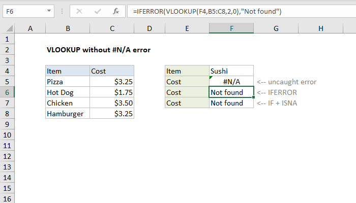
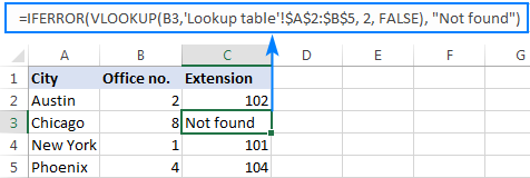
Example 1. IFERROR With Search By Formula To Change Errors With Your Own Text
If you want to replace the standard error notation with your own text, group the search by formula in IFERROR and enter the text in the client. wants in the 2nd argument (value_if_error), e.g. “Not found”:
Updated
Are you tired of your computer running slow? Annoyed by frustrating error messages? ASR Pro is the solution for you! Our recommended tool will quickly diagnose and repair Windows issues while dramatically increasing system performance. So don't wait any longer, download ASR Pro today!

VLOOKUP Returns Null Instead Of #N/A
The VLOOKUP function is one of the most useful functions for searching data with a specific range of cells in Excel. And if VLOOKUP doesn’t find a result, it looks for help and returns a #N/A error. And if you want to show “0” instead of #N/A. How to achieve this.
How To Change The Excel 2013 VLOOKUP Formula To Display Zero Instead Of #N/A
The following steps definitely assume that you already have a dominant VLOOKUP formula the formula is present in your worksheet, but you want to directly display “0” instead of #N/A. The formula will display #NA if it really can’t find the information it needs. By following the steps below, be will simply be replaced with “0”.
How It Works
If the IFERROR function does not work, you need to take the time to twosham. First, the value you want to evaluate for yourself, and second, each user you want to evaluate when an error occurs. Here is the syntax for IFERROR:
IFNA And VLOOKUP
If you use the VLOOKUP function to find a dollar value that somehow doesn’t exist in your search field, you should get an error #N/A. You can use the ifna function to change the error display to any message (or even an actual string) so that it is empty.
Syntax For Using The IFERROR Function
Leave me alone Let’s get started with a simple example of using the IFERROR function in Excel. To do this, column A is divided by column B, and the results can be displayed in columns C. See the formula and sample table below:
What Is IFERROR?
IFERROR is a function that is on the list of Excel logical functions among the most important Excel functions for financial analysts. This cheat site covers hundreds of features you know as an Excel category expert. IFERROR belongs to a group of functions that check for the presence ofsome errors, such as ISERROW, for example, ISERROW, ISERROW in combination with ISNA. The function returns a special output, usually set to a text string, when the calculation normally matches a formula with an error.
IFERROR With The VLOOKUP Function To Get Rid Of The #. NA The First Error Table Is The Original And Main Data, Desktop 2 Is The Vlookup Table. In Grin F, I Applied The Ingredient Recipe Using Vlookup To Find Laptop Sales By Brand.
IFERROR Function
Excel IFError function to recover the value of a when the formula returns with an error . For example, if we enter a lot in a formula cell and assume there is a certain chance of getting each error. In this case, we can use the IFERROR function to return something new each time the formula evaluates to an error.
#DIV/0! Errors
This can be seen when the last error number is divisible by 0. This is called a division error. Hovering over a cell with an error displays “Function is a DIVIDE parameter that cannot be null.”
Speed up your computer today with this simple download.Bästa Sättet Att Fixa Vlookup-fel 0
Лучший способ исправить ошибку Vlookup 0
Der Beste Weg, Um Den Vlookup-Fehler 0 Zu Beheben
La Mejor Manera De Corregir El Error 0 De Vlookup
Najlepszy Sposób Na Naprawienie Błędu Podglądu 0
Beste Manier Om Vlookup-fout 0 . Op Te Lossen
Meilleur Moyen De Corriger L’erreur Vlookup 0
Il Modo Migliore Per Correggere L’errore Vlookup 0
Melhor Maneira De Corrigir O Erro Vlookup 0
Vlookup 오류 0을 수정하는 가장 좋은 방법